1.Geoinformatics and Space Application Department, Centre for Environmental Planning and Technology (CEPT) University, Navrangpura, Ahmedabad, India; Geospatial Analyst
Cyient Europe Ltd
Reading, UK.
2.Geospatial Chair Professor, Center of Earth and Space Science, University of Hyderabad, Gachibouli, Hyderabad, India
*.Geoinformatics and Space Application Department, Centre for Environmental Planning and Technology (CEPT) University, Navrangpura, Ahmedabad, India; Geospatial Analyst
Cyient Europe Ltd
Reading, UK.
Indus valley has unique physiography and strategic significance for water resources and climate change impacts.
There was a gradual but significant rise in the built up area, a major reduction in the acreage of cultivated land with time.
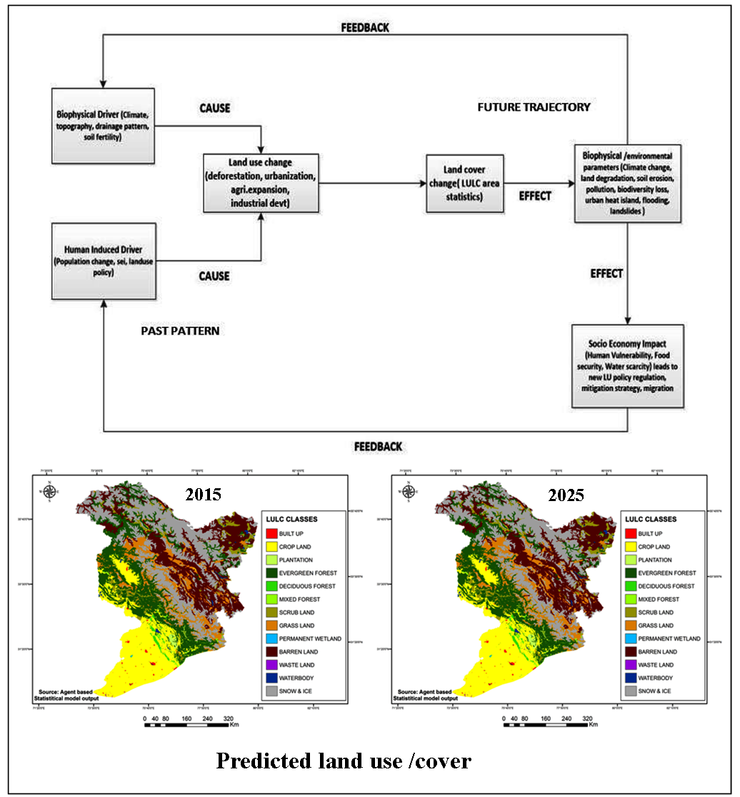
The study evaluates a dynamic land use simulation model developed to predict future land use scenarios of the basin on the basis of its past processes of change.
Physiographic and socio-economic drivers were used to predict the future land use land cover.
LULC classes over the basin area were modelled using a combination of transition probability and regression equation based on their past pattern of change with an average accuracy of 80 to 85%.
Abstract
The main objective of the present study is to project the future scenario of land use/ land cover on the basis of their past pattern of change. Indus basin with its diverse physiography is an ideal study area. Remote sensing sources from Landsat (MSS), LISS-I and LISS-III (1985–2005), were used to assess the past land use at a scale of 1:250,000. A statistical driver-based model was used to simulate the land use scenarios for 2015 and 2025. The model output was validated by comparing the simulated maps with reference ones for 2005 and 2015. All the land use classes displayed an overall accuracy of 85–90% with the exception of the classes “built-up” and “wasteland”.
Keywords
Transition probability , Multiple regression , Model Validation , Socio-economic change , Drivers of change , Land use/Land cover , Land use/land cover dynamics
1 . INTRODUCTION
Land use and land cover change is the basis for today’s alarming rate of global environmental change (Venter et al., 2016). It is the most critical issue in the study of environmental assessment because of its significant contributions to climate change, loss of habitat and biodiversity and improving standard of human life (Geoghegan et al., 2001). On a global scale, approximately 1.2 million km2 of land has been deforested and converted to various land uses in the last three centuries, while the agricultural land has increased by nearly 12 million km2 (Ramanakutty and Foley, 1999). Land use land cover dynamics is the major driver of any environmental change that has a direct implication on the soil moisture and atmospheric heat budget—the two most important components that shape the climate of a region (Boysen et al., 2014). Hence, these adverse environmental impacts of land use changes pose a critical challenge for all land use planners in designing sustainable economic growth. For assessing the impact of land use changes on the environment, the International Geosphere and Biosphere Program (IGBP) and International Human Dimensions Program (IHDP) on Global Environmental Change co-organized and endorsed research activity on land use land cover change scenarios (Geoghegan et al., 2001; IGBP, 1995).
The primary focus of the current study is modelling future land use scenarios based on their past pattern or drivers of change. Land use simulation based on their driver’s influence will provide a better understanding of land use systems identifying their pattern and help in prospective land use planning and policy (Soesbergen, 2015). A detailed understanding of future land use scenarios and potential environmental impacts will support land use planners and policy makers in making sound decisions and encourage them to practice sustainable land management so that a steady supply of natural resources is assured for future generations and the negative impacts of LULC change on the environment are alleviated (Aithal et al., 2013). Various
In general, the land use/land cover (LULC) of any region is defined and shaped by the environmental factors, such as climate, relief, vegetation and soil attributes (Verheye, 1998). But in recent years, both modification and conversion of any land use have been driven by human needs rather than natural changes (Turner et al., 1993). Thus most land use models have three key elements (Agarwal et al., 2001), of which time and space are the first two, providing a framework where all biotic and abiotic drivers interact. The human dimension of decision making is the third element of the model.
Literatures revealed that LULC models can be classified into three categories. The empirical-statistical models are the first group, such as regression models, which are developed by statistical analysis on the factors causing land use change (Pei and Pan, 2010). The spatially explicit models, are the second types simulating change based on transition rules such as the cellular automata model that represent transition rule based change but lack in their causal representation (Asranjani et al., 2013; Vaz et al., 2013). Thirdly, there are agent-based models, which simulate future scenarios based on factors of change also called agents but due to the multi-collinear behavior of the interacting agents, it seldom fails to represent the reality (Parker et al., 2003).
The current study entails a different approach of LULC modelling (statistical, spatial and driver-based approach) with quantitative simulation of future land use scenario at a river basin level, which analyses the processes of past decadal land use change (driver based) for the years 1985, 1995 and 2005 through statistical relations and representing the past pattern of change in the future at a temporal and spatial unit (spatially explicit approach).
Various researchers and environmentalists have assessed the trends of past land use dynamics and their ecological impacts at a local scale in various parts of the Indus river watershed. A forest fragmentation model was developed to characterize the changes in forest land use in the Mandhala watershed, in Himachal Pradesh (Ramachandra et al., 2012), from 1982 to 2007. Sonawane and Bhagat (2017) used simulation models for improved change detection of forested area. In a different study, multi-criterion decision analysis approach (Singh, and Andrabi, 2014) was utilized to find potential sites of urban development in the hilly terrain of Solan (HP), located in the current study area. The criteria were slope, aspect, elevation, transport network and land use/cover. The logistic regression technique was used in the land degradation study conducted by Gupta, and Sharma, (2010) to assess the impacts of various human drivers such as total owned land, land fragmentation, various levels of income, migration, labour availability, leasing out of land and literacy levels on the land degradation of the Himachal Himalayan zone. Human-induced factors such as population growth, urbanization and government policies were highlighted as the main drivers of change in Punjab from 1980 to 2010 (Adhikari and Shekhon, 2014). In another study, Rashid et al., (2015) confirmed the impacts of human-induced climate change on the receding glaciers of the Kashmir Himalaya through their study of the Kolohai glacier, Lidder valley. Kuchay et al., (2016) analysed the spatio-temporal impact of population growth and urban sprawl in the mountainous ecological background of Srinagar city.
Though several studies have been conducted at various times in the past at a local scale throughout the Indus watershed, the current study was the first of its kind in quantifying future land use processes on the basis of the past patterns of change, considering both physical and human drivers at a watershed level of analysis.
2 . STATISTICAL LULC MODELS
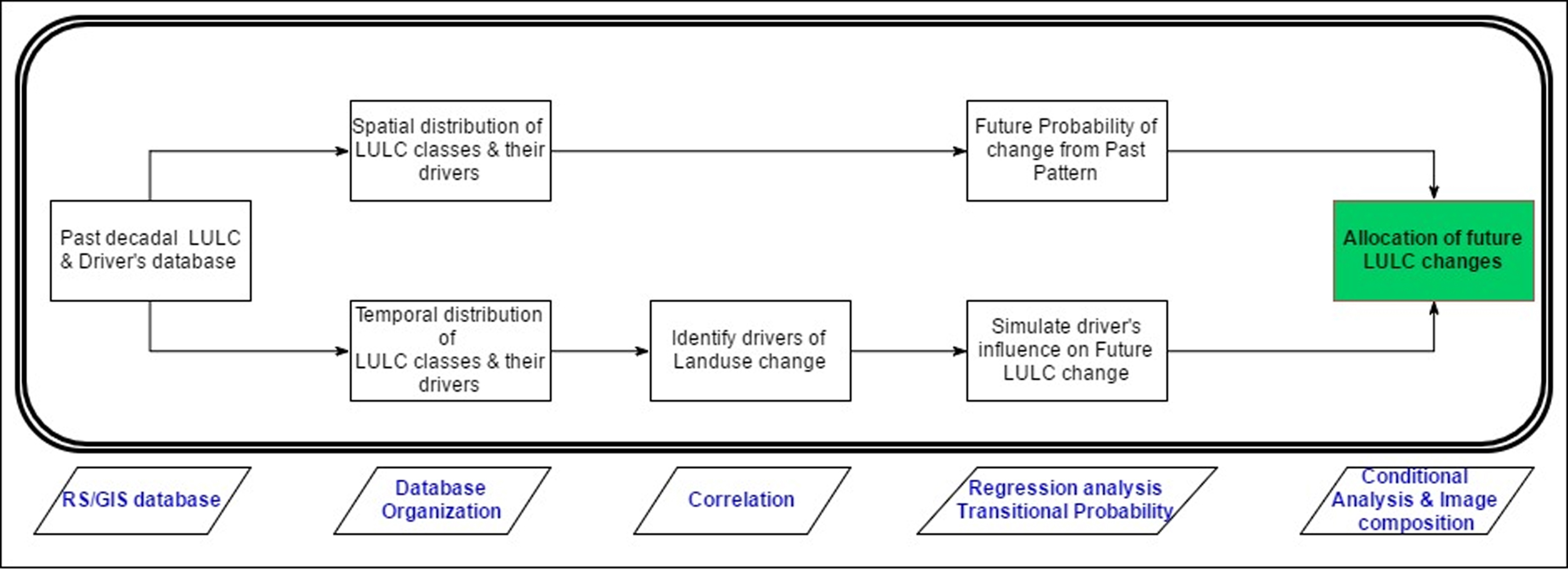
A statistical land use model has been applied in the current study, where multiple regressions were used to represent the impact of drivers on land use change, the transition probability of change was represented using Markov chain analysis. The spatial distribution of LULC was presented using a grid system with unique grid identifiers. The structure of the model is shown in figure 1.
Figure 1. Driver-based statistics model
2.1 Transition probability: the first component
Being a dynamic system, it represents the probability of a land use class that will change from one category to another or stay in the same, depending on the category at the initial time (Eastman et al., 2005). Such a model has at its center a transition matrix (A) that explains the likelihood of a cell changing from state i to state j (for all classes in the same discrete time step) and a vector (XT) displaying the frequency of each class at time t. A key assumption of transition models is that transition rates do not change over time (Peña et al., 2007). In the current study transition probability was used to estimate the probability of Land use change within a specified period of time.
2.2 Correlation Analysis: the second component
It signifies the degree to which two or more variables tend to vary together and therefore has an ability to measure the strength and direction of relationship between two variables (Torrico and Janssens, 2010; Kozak et al., 2012). It is estimated by dividing the sample covariance of variables by their standard deviation and is expressed in terms of the coefficient of correlation, r. The value of r ranges from -1 to +1 (i.e., -1< r < 1). The + and – signs are used for positive and negative correlation, respectively, and signify the direction of the relation between the variables.
A correlation matrix between Landuse classes (Y variable i.e. effect) with respect to their corresponding drivers of change (X variables i.e. causes) was generated and applied in the current model to identify the significant drivers for each LULC class change.
2.3 Regression Analysis: the third component
It represents the relationship between dependent and independent variables and is generally used to predict the behaviour of a dependent variable with respect to an independent one (Campbell and Campbell, 2008). Multiple regressions can ascertain that a set of independent variables has the ability to explain a proportion in a dependent variable at a significant scale of analysis and thus evaluate the predictability of the independent variables (Rawlings et al., 1998).
In the current model, regression analysis has been implemented to project the best fit relation between every landuse class (Y) and its corresponding selected set of non-collinear driver variables (X1 to Xn).
3 . STUDY AREA
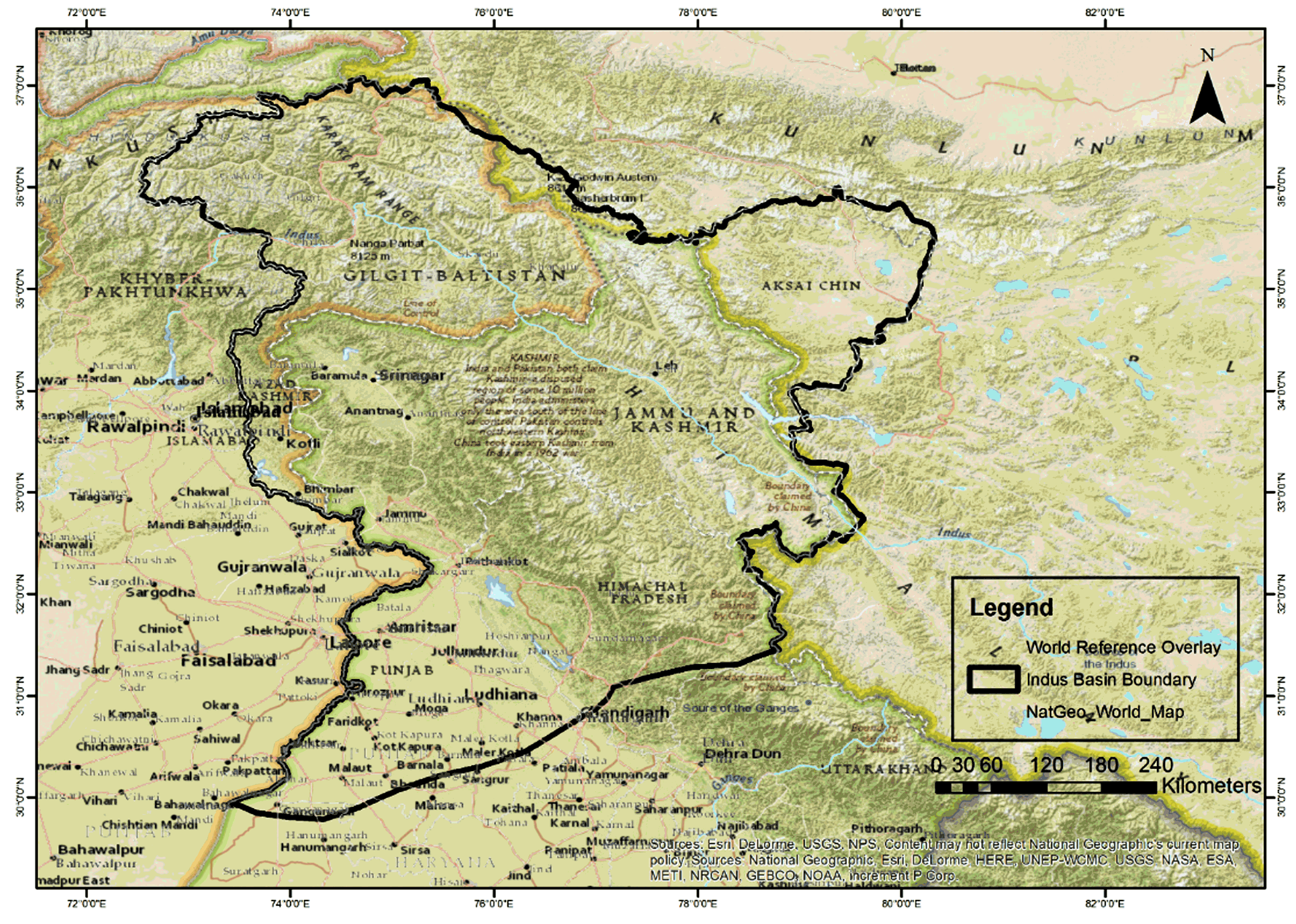
The Indus river basin extends over China (Tibet), India, Afghanistan and Pakistan, draining an area of 1,165,500 km2. The study area is the part of the Indus basin that lies within India (Figure 2). In India, the basin spreads over the states of Jammu & Kashmir, Himachal Pradesh and Punjab and parts of Rajasthan, Haryana and the union territory of Chandigarh. It has an area of 315,608 km2, covering 9.8% of the country’s geographical area. The basin is located between longitudes 72°28ʹ and 79°39ʹ E and latitudes 29°8ʹ and 36°59ʹ N. It covers a length of 756 km and a width of 560 km. The basin is surrounded by the Himalaya, in the east, the Karakoram ranges, in the north, the Kirthar and Sulaiman ranges, in the west, and the Arabian Sea, in the south (Indus River).
Figure 2. Study area: the Indus river basin in India
The major part of the basin is covered with agricultural land, which accounts for 35.8% of the total area, and 1.85% of the basin is covered by waterbodies. The upper part of the basin consists mostly of mountain ranges with steep slopes and narrow valleys in the states of Jammu & Kashmir and Himachal Pradesh. The lower part of the basin is situated in Punjab, Haryana and Rajasthan and consists of vast plains covered with fertile alluvium. The major soil types found in the basin are sub-montane, alluvial soils and brown hill. The cultivable area of the basin is about 9.6 million ha, which forms 4.9% of the total cultivable area of the country.
The important urban centers and towns in the basin are Chandigarh, Srinagar, Ambala, Patiala, Bathinda and Shimla. Industrial growth in the basin is based on agricultural equipment and agriculture-based products such as textiles, wool, sugar and paper. Being a hill economy and given its distance from the main markets in India, transportation costs are high. Intensive cultivation is practiced because of the constraints of the cultivable land available. Irrigation and high-yielding seeds are important for cultivation. Both the human and livestock populations directly depend on the forest for survival. Under the pressure of urbanization, the increasing population encroach the forest for housing and agriculture purpose. Tourism is the most popular service industry of the state depending on its aesthetic beauty of mountains, valleys, lakes, and the coniferous canopy. The fragile ecology and the high cost of accessibility in the northern part of the basin hinder the growth of any large-scale industry.
Due to the high variability in the climatic parameters (temperature ranging from 30°C to sub-zero temperatures, rainfall ranging from as low as 15 mm to 3000 mm) and topographic features (rugged Himalayan topography to level land) and variations in the spatial and temporal impacts of human influence, the Indus basin is ideal for studying the effects of natural and human drivers on the changing land cover of the Earth. No attempt to study and identify the significant land use and its drivers of change to assess its environmental impact of the Indus basin in India has been undertaken earlier.
4 . MATERIALS AND METHODOLOGY
4.1 Data input for the model
4.1.1 Past Land use/land cover dataset
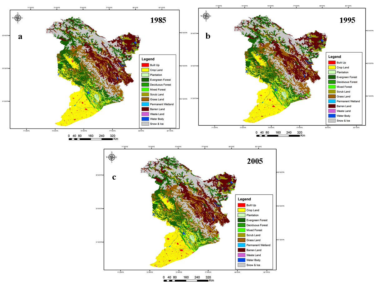
The vector LULC database created from the geo-rectified satellite data of Landsat MSS, IRS LISS-I and IRS LISS-III, were used to produce raster LULC datasets (Figure 3) for the years 2005, 1995 and 1985 (at decadal interval), at a spatial resolution of 125 m. Based on IGBP level II classification scheme 13 landuse/ landcover classes were identified during the period (Built up, crop land, plantation, evergreen forest, deciduous forest, mixed forest, scrub land, grass land, permanent wetland, barren land, waste land, waterbody and snow and ice).
Figure 3. Decadal LULC of Indus river basin: a) 1985, b) 1995 and c) 2005
4.1.2 Driver datasets
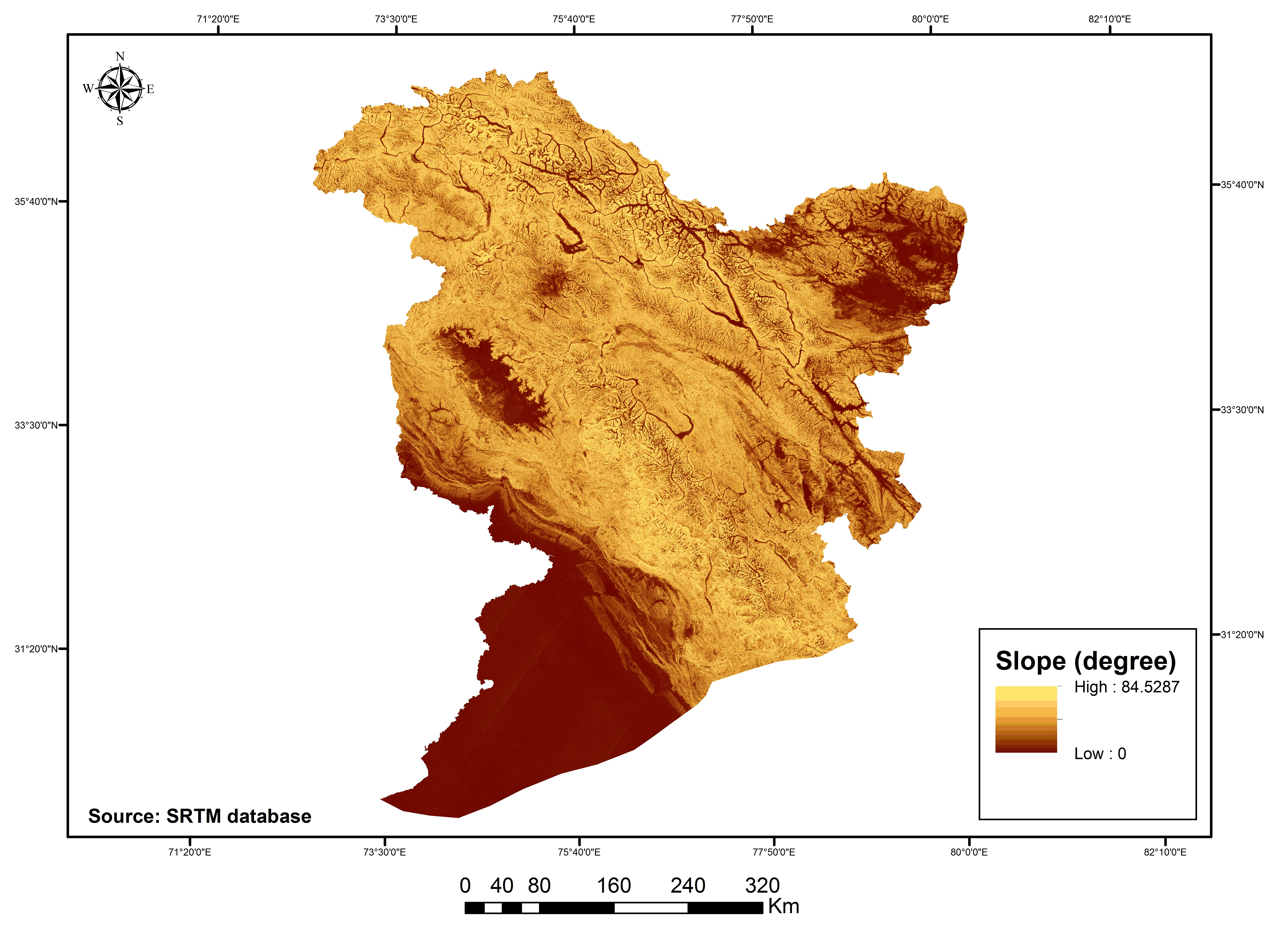
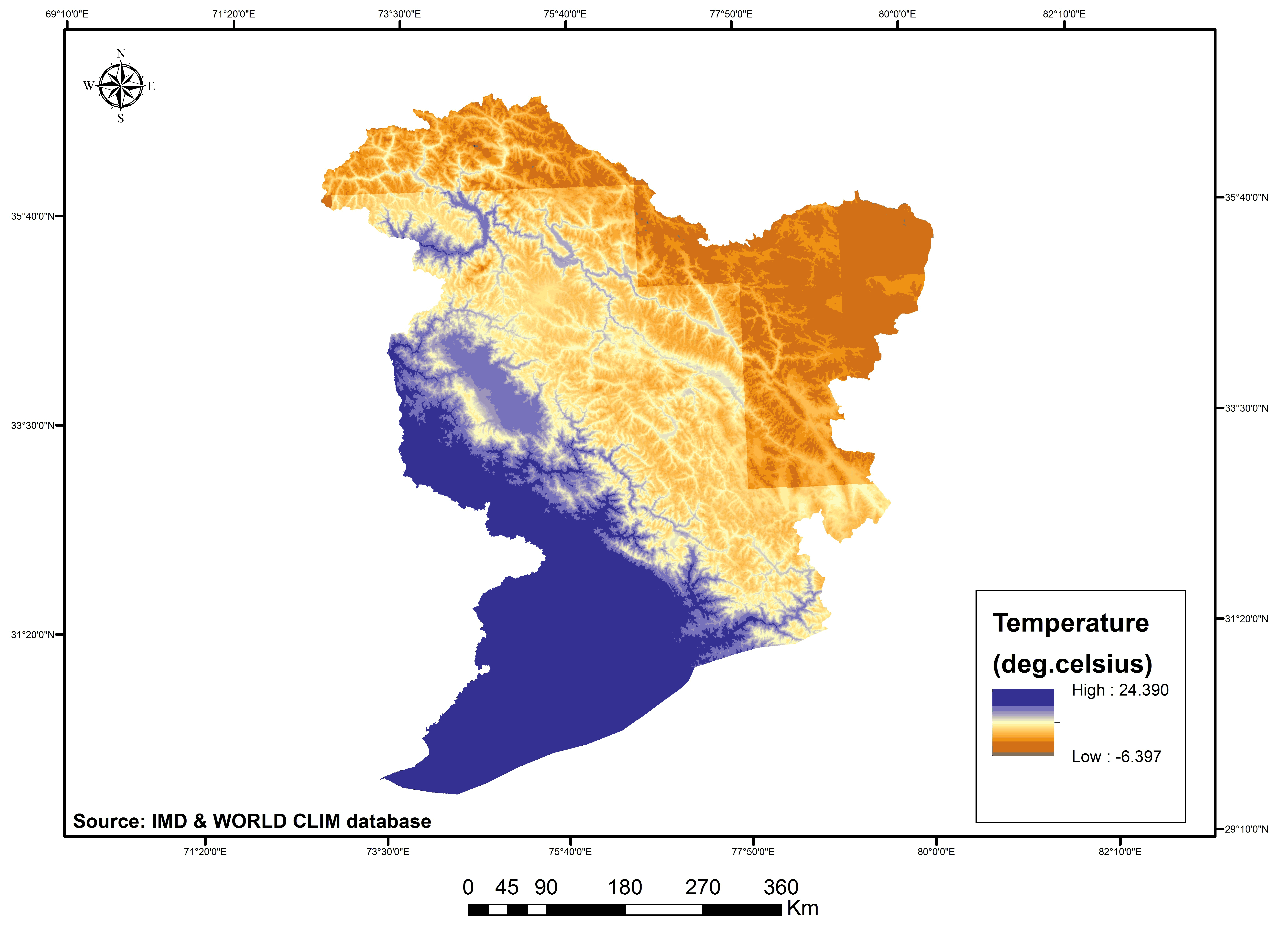
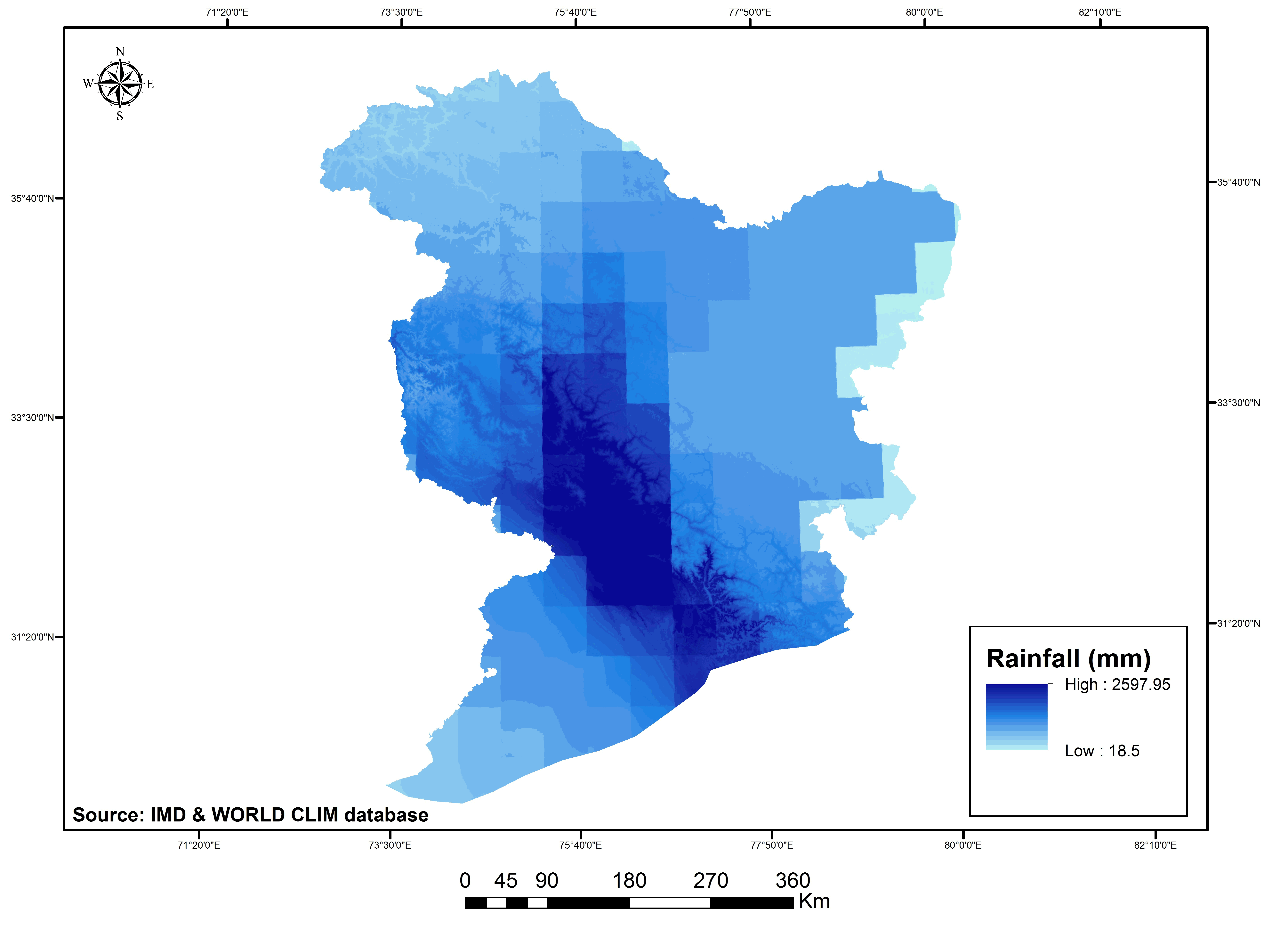
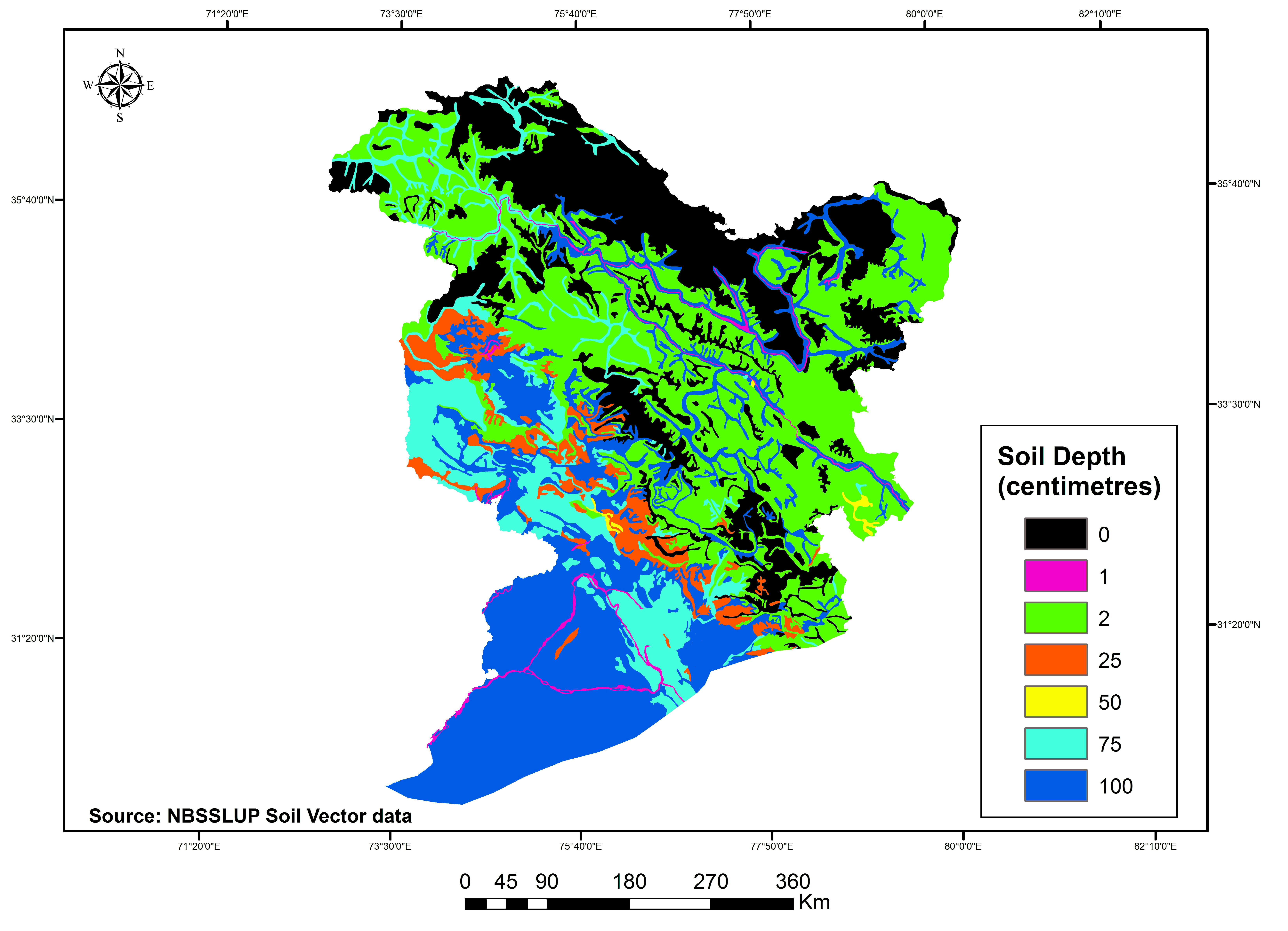
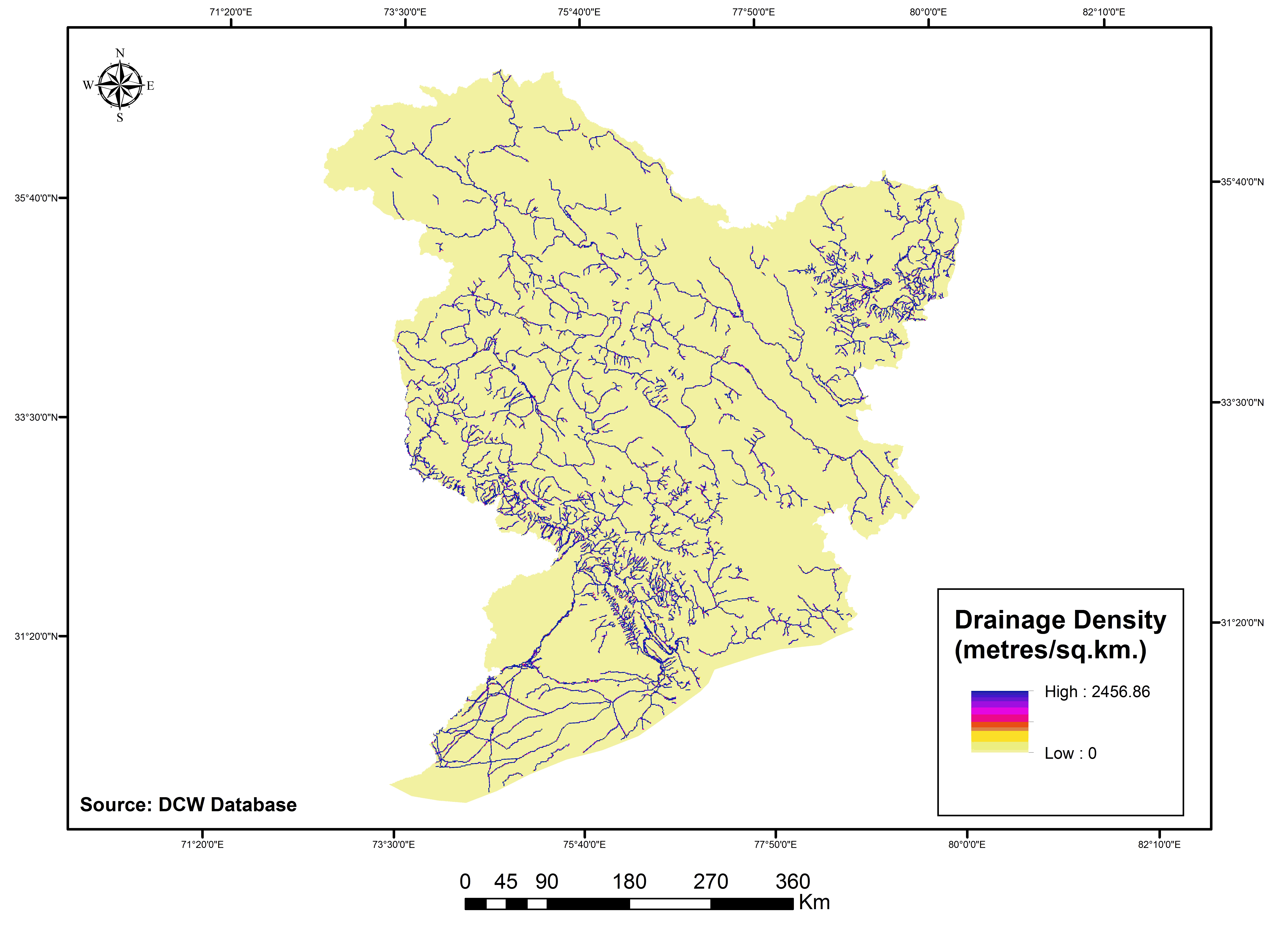
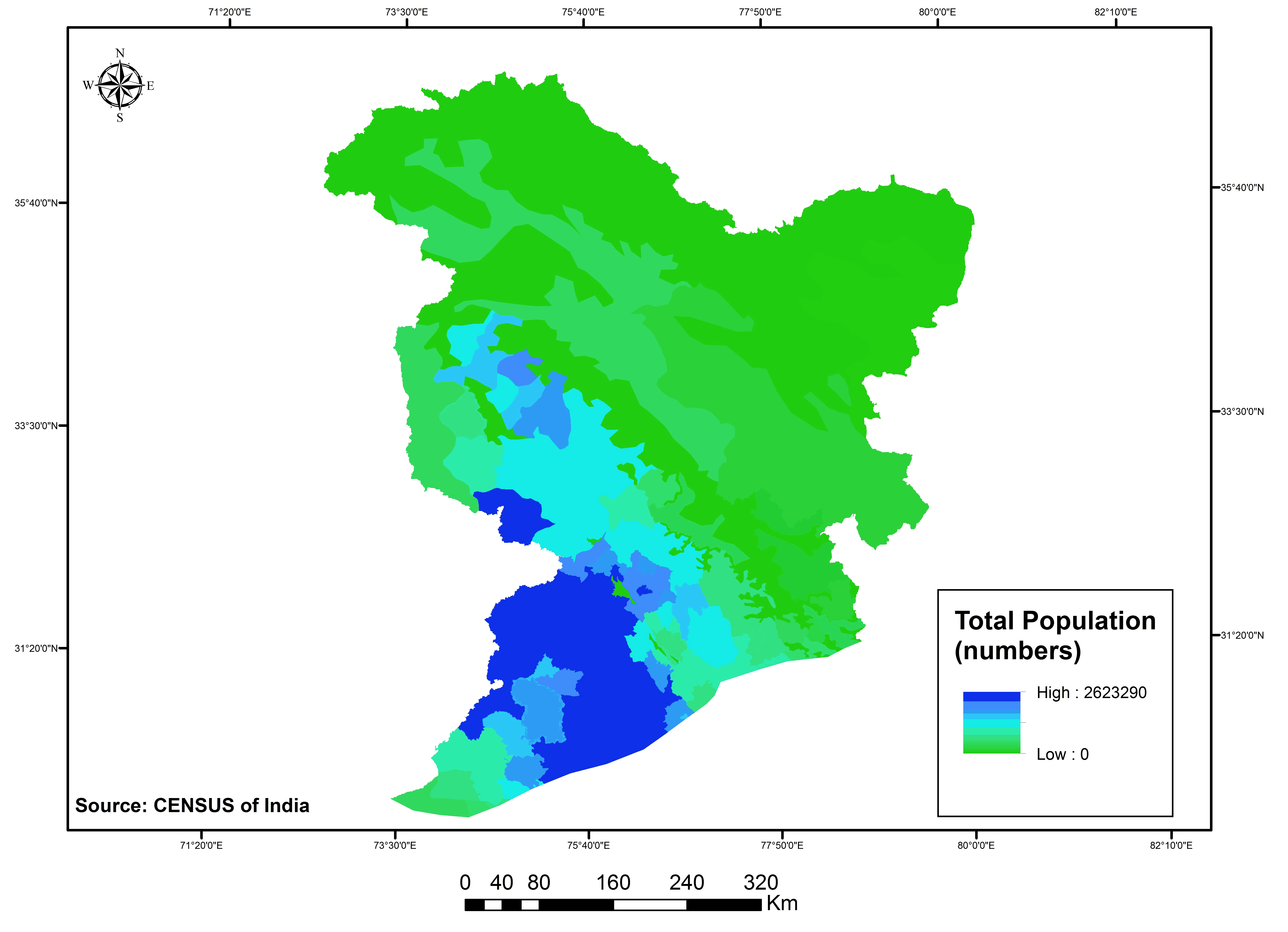
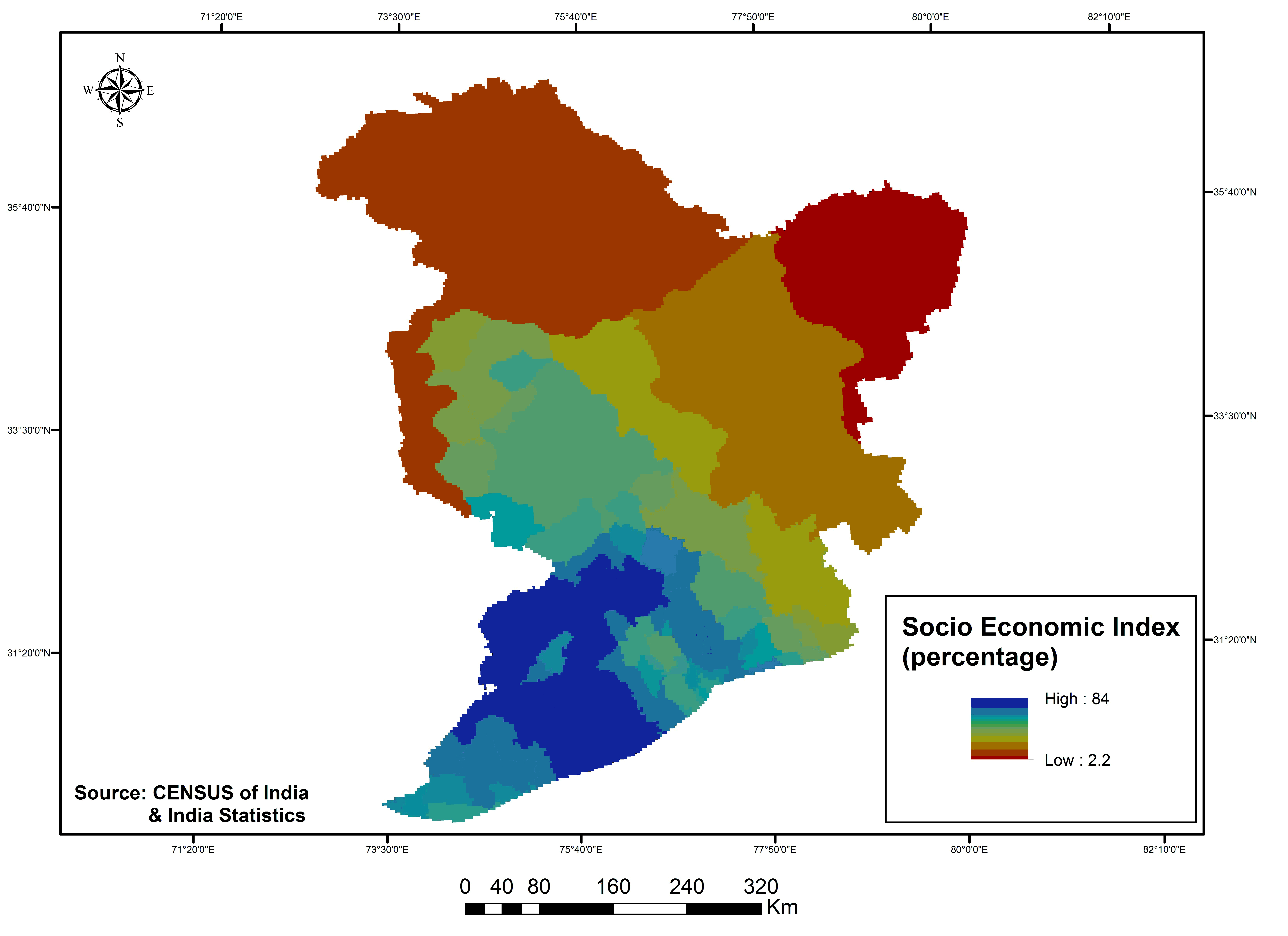
The physical (elevation, slope, soil depth, mean monthly temperature, mean annual rainfall and drainage density) and human (taluk wise total population and socio economic parameters like working population, literacy rate, drinking water facility, sex ratio, road length represented as socio economic index ) drivers’ data were collected, and organized for those corresponding years of 1985, 1995 and 2005 from various sources (Digital Elevation Model, National Bureau of Soil Survey & Land use Planning Soil map, Indian Meteorogical Data, Digital Chart of the world, Census of India, India stat report) and in different resolutions. To analyse and assess them in a model set-up, it was necessary to convert each driver data to raster format (example shown in figure 4 and 5 with a 125m spatial resolution. Thereby to avoid the modifiable aerial unit problem and for the sake of unbiased analysis, data were resampled at a uniform spatial level and was aligned in the same format, having the same projection and resolution parameters as those of the LULC raster maps.
Figure 4a. Physical drivers: Slope
Figure 4b. Physical drivers: mean annual temperature
Figure 4c. Physical drivers: Rainfall
Figure 4d. Physical drivers: Soil depth
Figure 4e. Physical drivers: Drainage density
Figure 5a. Human induced drivers (2005): Total population
Figure 5b. Human induced drivers (2005): Socio-economic Index
4.1.3 Grid mesh (vector layer)
Unlike CA model, where the spatial representation of land use change depends on the local influences of the neighbouring land use cells, the current model considers a grid system to spatially project the future pattern of land use change in each grid. The grid system consisted of a grid mesh covering the entire study area, i.e., 315,608 km2 (Indus watershed area in India) and was composed of individual grid cells of a particular chosen dimension represented by grid id. For the study area, since both the land use and driver database rasters were at a resolution of 125 m, a larger grid size of 1 km/1 km was considered to represent the future land use scenario.
4.2 Methodology used
The LULC modelling in the Indus watershed was carried out with six different steps, namely, temporal analysis, data preparation, driver selection, predicted output, thematic image composition and composite output.
4.2.1 Temporal analysis
The temporal complexity of land use change is analysed in terms of the probability of a transition from one class to another in a given time period. The Markov analysis was utilized to generate the rate of land use change between two time periods (Table 1), where the inputs were the two raster LULC images for the initial year and the base year (T0 and T1). Based on the initial and base year, future landuse was estimated for 2015 and 2025 (T2). For the prediction for 2015, the transitional probability (TP) for the period from 1995 to 2005 (since T0 = 1995 and T1 = 2005) was generated and for 2025, the TP for the period from 1985 to 2005 was used (as T2 = (T1 - T0) + T1).
Table 1. Transitional probability matrix (1985, 1995 and 2005)
1985-1995
BU
CL
PL
EF
DF
MF
SL
GL
PW
BL
WL
WB
SI
BU
0.92
0.04
-
-
0.01
-
0.02
-
-
-
0.01
-
-
CL
0.01
0.99
-
-
-
-
-
-
-
-
-
0.02
-
PL
-
-
1
-
-
-
-
-
-
-
-
-
-
EF
-
-
-
0.95
-
-
0.01
0.01
-
0.02
-
-
0.01
DF
-
-
-
0.01
0.93
-
-
-
-
-
-
-
-
MF
-
-
-
0.01
-
0.95
0.02
-
-
0.01
-
-
0.01
SL
-
-
-
0.01
-
-
0.97
0.01
-
0.01
-
-
0.01
GL
-
-
-
0.01
-
0.01
0.02
0.9
-
0.04
-
-
0.03
PW
-
-
-
-
-
-
-
-
1
-
-
-
-
BL
-
-
-
0.01
-
-
0.01
0.01
-
0.94
-
0.01
0.03
WL
-
0.04
-
-
-
-
-
-
-
-
0.96
-
0
WB
-
0.01
-
-
-
-
-
-
-
0.01
-
0.98
0.01
SI
-
-
-
0.01
-
-
-
0.02
-
0.03
-
-
0.94
1985-2005
BU
CL
PL
EF
DF
MF
SL
GL
PW
BL
WL
WB
SI
BU
0.93
0.05
-
-
0.01
-
0.01
-
-
-
0.01
-
-
CL
0.02
0.97
-
-
-
0.01
-
-
-
-
-
0.01
-
PL
-
-
1
-
-
-
-
-
-
-
-
-
-
EF
-
-
-
0.9
-
-
0.01
0.04
-
0.02
-
-
0.03
DF
-
-
-
-
0.92
0.01
-
-
-
-
-
0.01
-
MF
-
-
-
0.01
-
0.94
0.01
0.02
-
-
-
0.01
-
SL
-
-
-
0.01
-
-
0.93
0.03
-
0.01
-
-
0.02
GL
-
0.01
-
0.01
-
0.01
0.02
0.86
-
0.05
-
-
0.05
PW
-
-
-
-
-
-
-
-
1
-
-
-
-
BL
-
-
-
-
-
-
0.01
0.01
-
0.93
-
-
0.04
WL
0.02
0.13
-
-
-
-
-
-
-
-
0.86
-
-
WB
-
0.01
-
-
-
-
-
-
-
-
-
0.99
-
SI
-
-
-
-
-
-
0.01
0.05
-
0.04
-
-
0.89
1995-2005
BU
CL
PL
EF
DF
MF
SL
GL
PW
BL
WL
WB
SI
BU
0.96
0.04
-
-
0.01
-
-
-
-
-
-
-
-
CL
0.02
0.98
-
-
-
-
-
-
-
-
-
-
-
PL
-
-
1
-
-
-
-
-
-
-
-
-
-
EF
-
-
-
0.93
-
-
0.01
0.02
-
0.02
-
-
0.02
DF
-
-
-
-
0.99
0.01
-
-
-
-
-
0.01
-
MF
-
-
-
0.01
-
0.98
-
0.01
-
-
-
-
-
SL
-
0.01
-
0.01
-
0.01
0.88
0.06
-
0.03
-
-
0.02
GL
-
0.01
-
-
-
-
0.01
0.9
-
0.04
-
-
0.04
PW
-
-
-
-
-
-
-
-
1
-
-
-
-
BL
-
-
-
-
-
-
0.02
0.04
-
0.91
-
-
0.03
WL
0.02
0.2
-
-
-
-
-
-
-
-
0.78
-
-
WB
-
0.01
-
-
-
-
-
-
-
0.01
-
0.99
-
SI
-
-
-
-
-
-
0.01
0.04
-
0.03
-
-
0.92
4.2.2 Preparation of database
The second step was to organize both database (land use and drivers) in a similar format for convenience of modelling. Since grid cells are used to spatially represent the future land use scenario, thereby both the input databases were organized and distributed in 1km grid cells, with their grid identities as unique identifier and their corresponding values as an attribute to each cell. Using mean function of zonal statistics and tabulate area, input data were distributed in each vector grid cell.
4.2.3 Driver selection
The drivers affect the land use classes in various ways. A driver that is highly related and effective for one land use class may not be equally significant for another since land use classes are not affected in the same manner by all the drivers. For instance, the built-up land use will be highly dependent on a demographic driver like population growth, but it will not be affected as much by the drainage density of the region. Thus identifying and locating the set of influential drivers for a particular land use was the next step that will be the major input in the prediction process. This was accomplished by the correlation statistics between the LULC distribution and their corresponding drivers of change for each taluk (Table 2) at a significance level of 0.05 with the minimum threshold at r>= 0.138 (with degree of freedom= 121), that displays the correlation coefficient (r) of each land use–driver pair, representing the direction (direct or inverse proportionality) and strength of the relation between them. The value of r is the basis on which drivers are selected for each land use category, higher the value (positive or negative highlighted in bold) greater is the LU-driver dependence. Approximately two to five non collinear drivers having consistent impact over three years had been considered for each land use class.
Table 2. Correlation matrix (land use vs drivers) at alpha = 0.05
1985
Elevation (m)
Soil-depth (cm)
Slope (degree)
Population
SEI
(%)
DD
(m/km2)
Temperature (C)
Rainfall (mm)
BU
-0.287
0.235
-0.387
0.456
0.369
-0.047
0.243
-0.282
CL
-0.517
0.434
-0.638
0.681
0.570
-0.132
0.531
-0.416
PL
-0.057
-0.011
0.069
-0.135
-0.116
0.342
0.036
0.387
EF
0.376
-0.345
0.336
-0.272
-0.431
-0.083
-0.436
-0.060
DF
-0.217
0.102
-0.206
0.173
0.150
0.420
0.176
0.214
MF
0.267
-0.351
0.318
-0.319
-0.325
0.149
-0.285
0.184
SL
0.368
-0.319
0.167
-0.272
-0.459
-0.040
-0.401
-0.143
GL
0.606
-0.564
0.342
-0.337
-0.506
-0.154
-0.622
-0.235
PW
-0.176
0.146
-0.210
0.220
0.107
0.041
0.191
-0.117
BL
0.442
-0.391
0.146
-0.247
-0.437
-0.100
-0.443
-0.215
WL
-0.247
0.144
-0.280
-0.068
0.119
0.280
0.261
-0.078
WB
-0.071
-0.030
-0.313
0.149
-0.057
0.276
0.029
-0.166
SI
0.524
-0.490
0.302
-0.306
-0.495
-0.130
-0.537
-0.214
1995
BU
-0.224
0.199
-0.338
0.379
0.246
-0.070
0.184
-0.247
CL
-0.516
0.425
-0.626
0.618
0.486
-0.111
0.528
-0.448
PL
-0.057
-0.011
0.070
-0.129
-0.037
0.334
0.033
0.312
EF
0.370
-0.338
0.330
-0.233
-0.442
-0.082
-0.432
-0.018
DF
-0.215
0.100
-0.203
0.188
0.178
0.410
0.171
0.268
MF
0.285
-0.369
0.309
-0.262
-0.284
0.134
-0.301
0.198
SL
0.365
-0.308
0.153
-0.229
-0.427
-0.060
-0.403
-0.109
GL
0.581
-0.538
0.326
-0.311
-0.505
-0.138
-0.584
-0.155
PW
-0.176
0.146
-0.210
0.198
0.089
0.039
0.189
-0.167
BL
0.461
-0.421
0.185
-0.256
-0.465
-0.119
-0.478
-0.163
WL
-0.239
0.170
-0.281
-0.183
0.042
0.088
0.272
-0.225
WB
-0.081
-0.022
-0.320
0.202
-0.074
0.286
0.006
-0.123
SI
0.553
-0.508
0.278
-0.307
-0.560
-0.112
-0.589
-0.171
2005
BU
-0.370
0.295
-0.482
0.554
0.392
-0.157
0.334
-0.393
CL
-0.505
0.419
-0.622
0.630
0.482
-0.133
0.494
-0.453
PL
-0.057
-0.011
0.070
-0.142
-0.023
0.335
0.039
0.278
EF
0.369
-0.339
0.339
-0.231
-0.423
-0.076
-0.465
-0.026
DF
-0.215
0.099
-0.204
0.179
0.184
0.410
0.170
0.221
MF
0.286
-0.317
0.350
-0.294
-0.268
0.093
-0.290
0.216
SL
0.399
-0.340
0.186
-0.259
-0.510
-0.031
-0.543
-0.120
GL
0.620
-0.582
0.373
-0.317
-0.502
-0.139
-0.649
-0.155
PW
-0.176
0.146
-0.210
0.197
0.100
0.025
0.183
-0.143
BL
0.486
-0.436
0.180
-0.268
-0.453
-0.101
-0.558
-0.189
WL
-0.235
0.161
-0.275
-0.183
-0.092
0.077
0.254
-0.212
WB
-0.055
-0.042
-0.299
0.178
-0.086
0.259
-0.090
-0.188
SI
0.544
-0.499
0.271
-0.303
-0.528
-0.105
-0.634
-0.182
4.2.4 Land use prediction
The next step performs prediction analysis using the regression technique. The significant drivers identified for each land use category were used as the major input projecting the best-fit relation in terms of their level of significance on the respective land use class. According to their correlation coefficient, the set of drivers are inserted in the regression equation as the independent X variables to estimate the predicted Y (land use/dependent variable). For both, 2015 and 2025, the base year (T1) of prediction was 2005. Hence regression analysis was carried out on the datasets for 2005 (land use and drivers) because of the data availability.
LU class pred(2005) = a ± b1Dr1 ± b2Dr2 ± b3Dr3 ± ………
(DF) pred = a ± 0.3 * rain ± 0.24 * elev ± …………,
where a = intercept value (output of regression) and
b (1, 2, 3…n) = slope coefficient (output of regression).
This section of the modelling not only predicts Y at T1 but also ensures the significance of the predicted land use class Y using the SEOE (Standard Error of Estimate). All the predictions were accepted at the ±1 SEOE (90%) level of significance.
At the final step, the predicted area of each land use (regression output) for T1 (2005) was multiplied by their respective transition probabilities for the corresponding time period to simulate their areal distribution for T2 (2015 or 2025). For prediction for 2015, the TP of the period 1995–2005 was considered, while the TP of 1985–2005 was used in the calculation for 2025. Thereby for each future land use class, area is calculated for each 1km grid as the product of predicted area for that class in 2005 (regression output) and its corresponding transition probability (change pattern from different classes).
Predicted LU class 1(2025) = Predicted LU class1 (2005) * TP (1985–2005)
Predicted LU class 1(2015) = Predicted LU class1 (2005) * TP (1995–2005)
Finally the future LULC area under the 13 land use classes within the basin was organized in tabular format with respect to their grid identifiers and spatial information, for both 2015 and 2025.
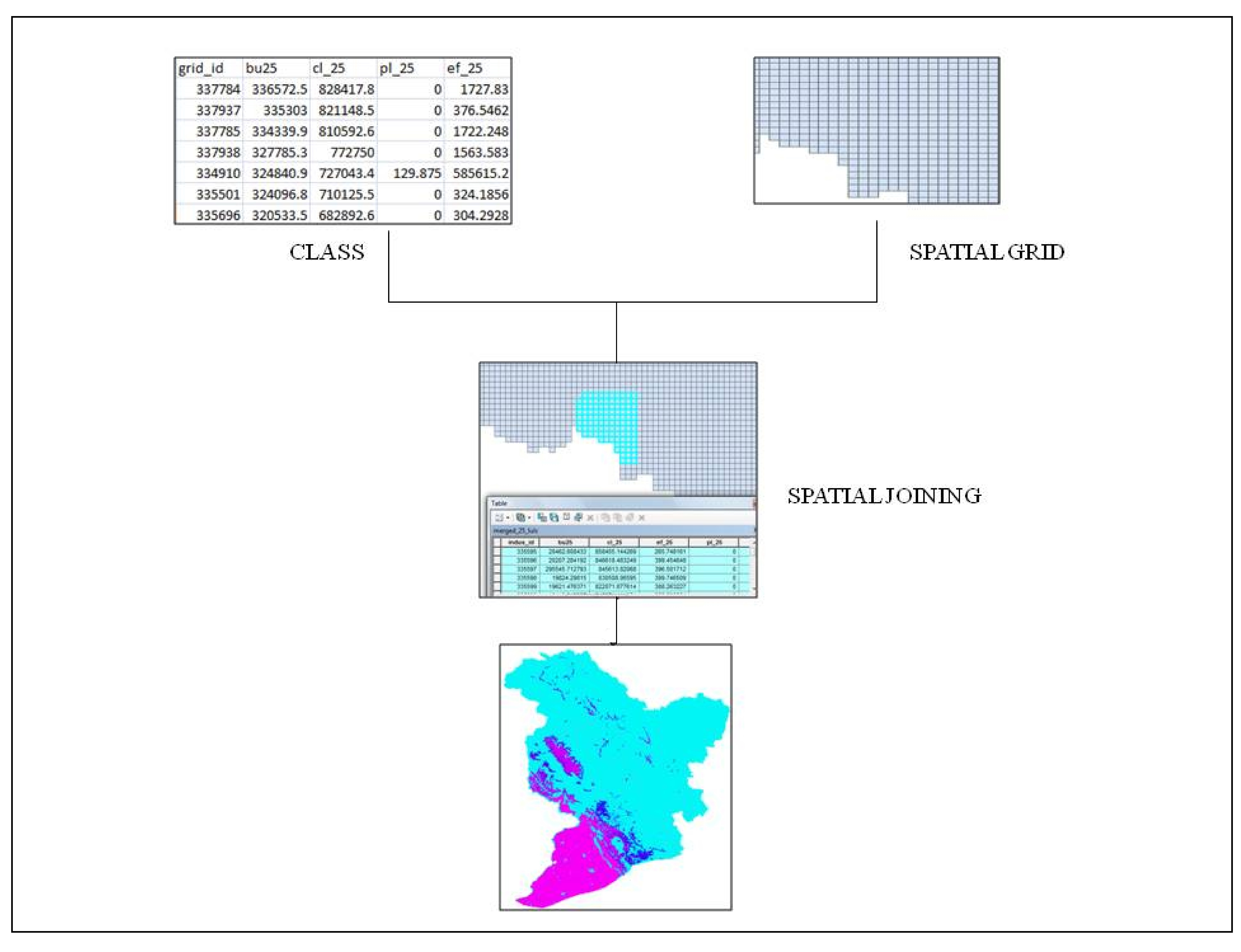
All the input data were organised in grid vector with respect to the grid identifiers as their spatial coordinates. As a result, the model displays the output data for each land use class for each cell in a tabular format. These tables, with their respective grid identifiers and land use area statistics, were then converted into the thematic rasters by rasterizing the grid vector using the land use area field for each class at a time (Figure 6). Thirteen thematic maps, one for each land use class, were generated for 2015 and for 2025. This process not only preserves the geographic locations of the land use classes in the study area and their sizes but also can detect the minor changes in any land use class. A similar approach has been used in the Land Transformation Model by Pijanowski et al., (1995, 1996).
Figure 6. Schematic preparation of a land use map
4.2.6 Composite land use map generation
In order to generate a single composite of all the thematic layers (land use classes), a composite image was created in the final step that includes all the predicted land use classes for T2 (2015 and 2025). The composite image was generated in the spatial modeller by applying the majority conditional decision rule to it.
5 . RESULTS: PREDICTION OUTPUT
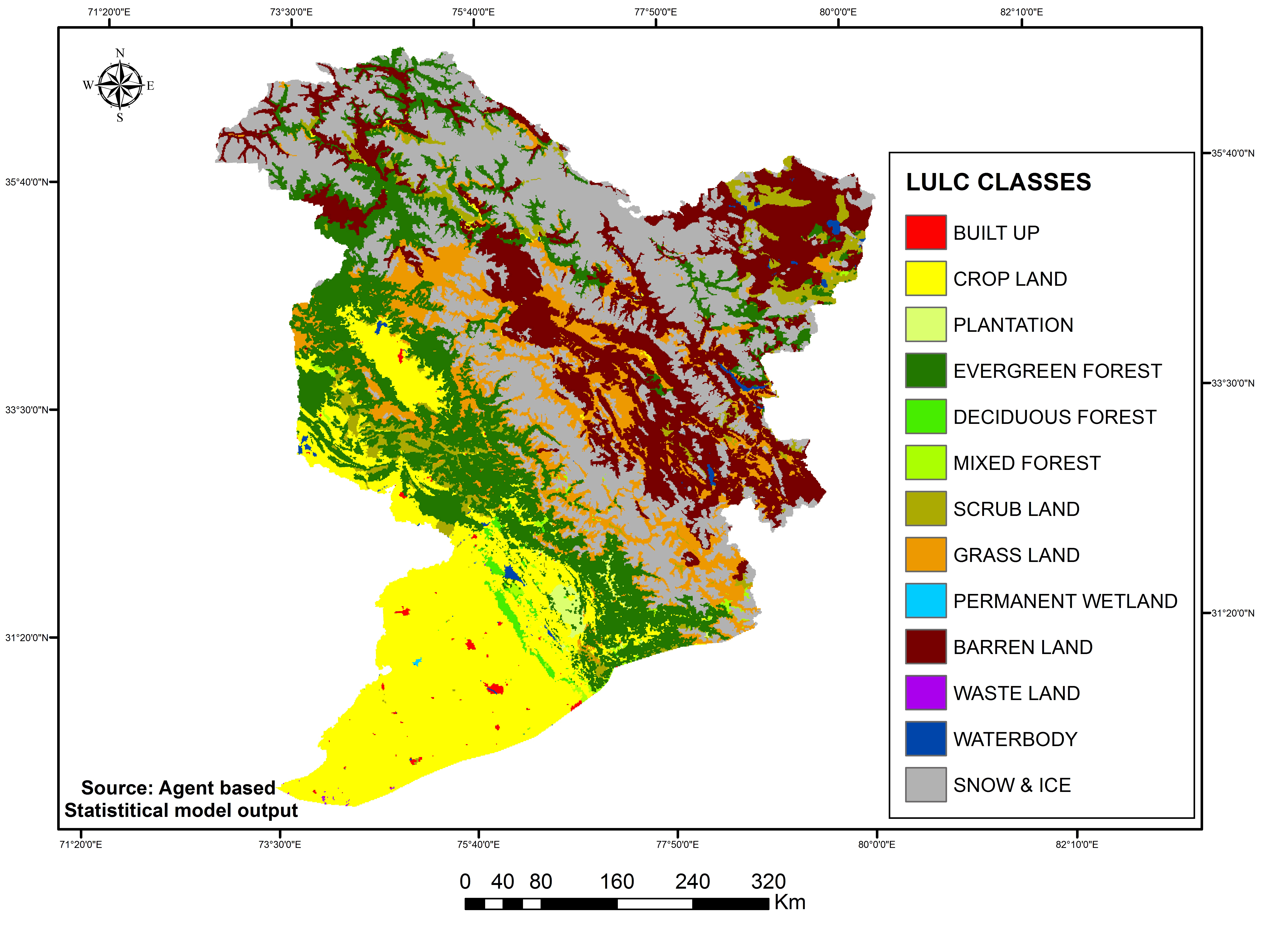
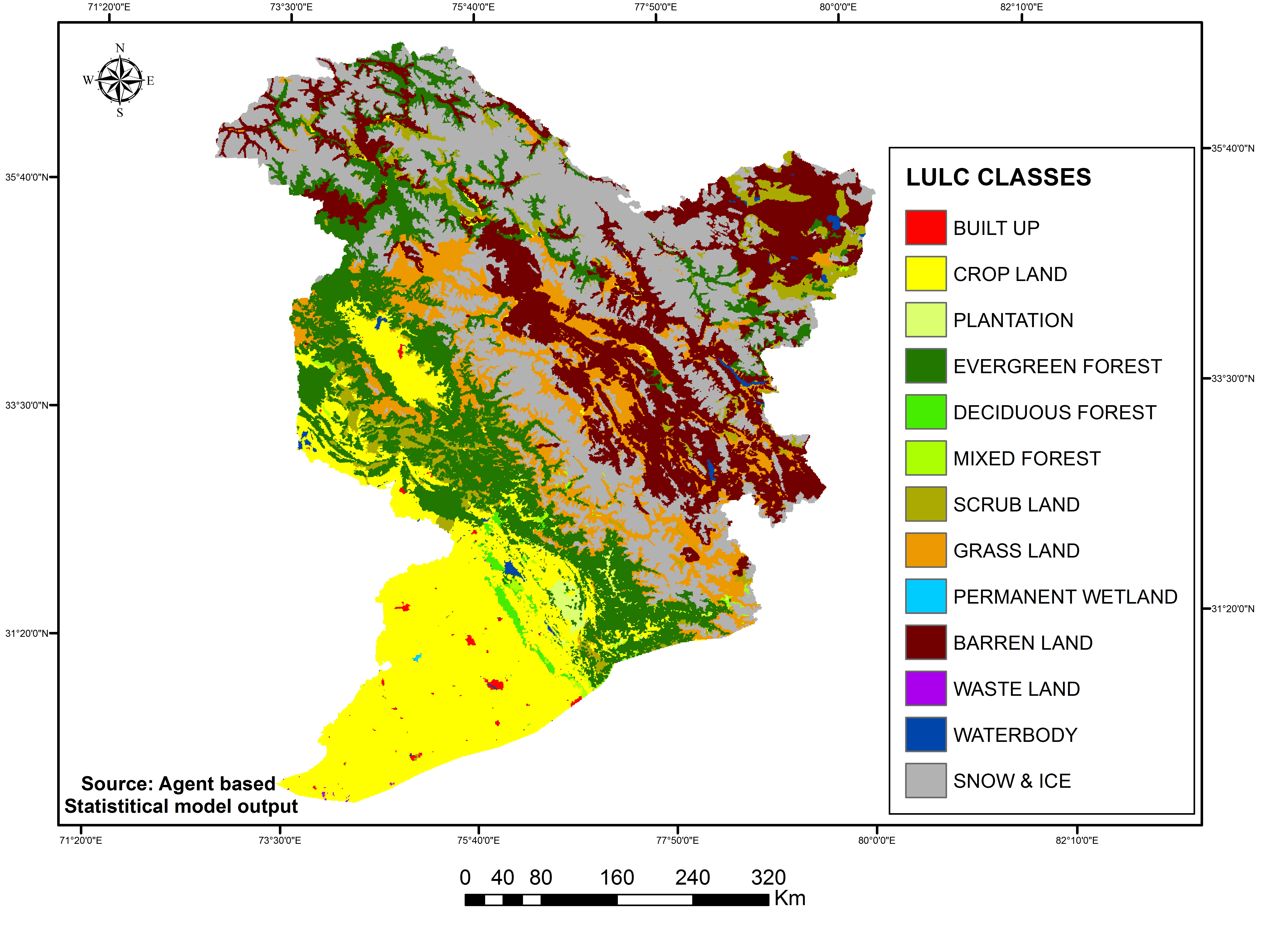
A hybrid driver-based statistical modelling of the study area (315,608 km2) using the methodology described was carried out to generate area statistics of the land use classes and generate land use thematic maps for 2015 and 2025. The inputs of the model, i.e., the database of the past land use and the corresponding driver database, were used in raster format at the same spatial resolution (125m). To make predictions for 2015 and 2025, the land use datasets of 1995-2005 and 1985-2005 (T0 and T1, respectively) were used as the inputs. The composite LULC map for 2015 and 2025 is shown in figure 7. The area statistics of each land use class for the predicted years are presented in Table 3 and figure 8.
Figure 7a. Predicted LULC: 2015
Figure 7b. Predicted LULC: 2025
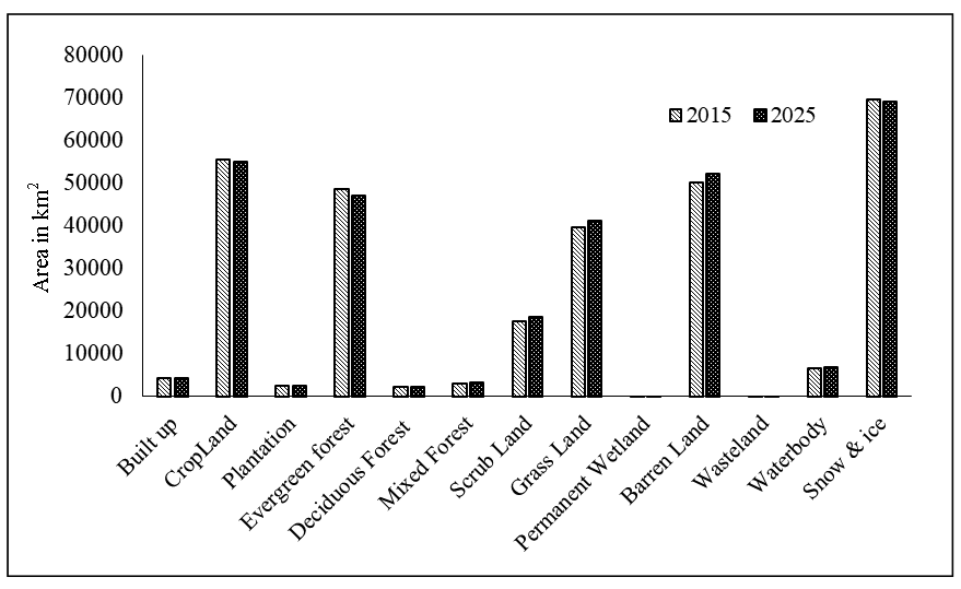
Figure 8. Predicted LULC
6 . CALIBRATION AND VALIDATION OF MODEL
In the current model for Indus LULC, the input predictor variable (drivers) were selected on the basis of their significance of influence i.e. correlation coefficient (r, Table 1) on the corresponding land use class. Secondly drivers with high multi-collinearity (higher dependency on each other), determined by their correlation coefficient (>0.8) according to Menerd (2001), were excluded from the model to avoid their impact on the standard error of regression coefficient, (Yoo et al., 2014).
Another crucial aspect of model validation was the issue of spatial autocorrelation among the chosen input data. In most of the cases, studies with spatial data are attributed by some degree of spatial autocorrelation which represent the influence of surrounding land use on the land cover at a particular location (Brown et al., 2002; Rutherford et al., 2008). Spatial autocorrelation in the data affects the regression model by biased estimation of error variance, t-test significance level and over estimation of R2 (Anselin and Griffith, 1988). In the current model, for reducing the impact of spatial autocorrelation, spatially lagged variables has been considered as the model input (Lasschen et al., 2005). Each lagged variable is the average (zonal mean) of the values of the original variable in surrounding 8/8 cells of its location. Thus all the variables used as model predictor were spatially lagged of their original values, hence reducing the local impact of land use on the land cover scenario.
Impact of driver variables on the land use has already been tested by the significance of correlation coefficient at a 95 % significance level. SEOE was used for validating the model output, where the prediction values (land use classes) has been restricted to +/-1SEOE providing significance of prediction at 90% level of significance.
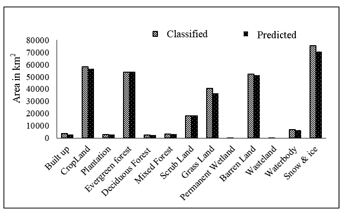
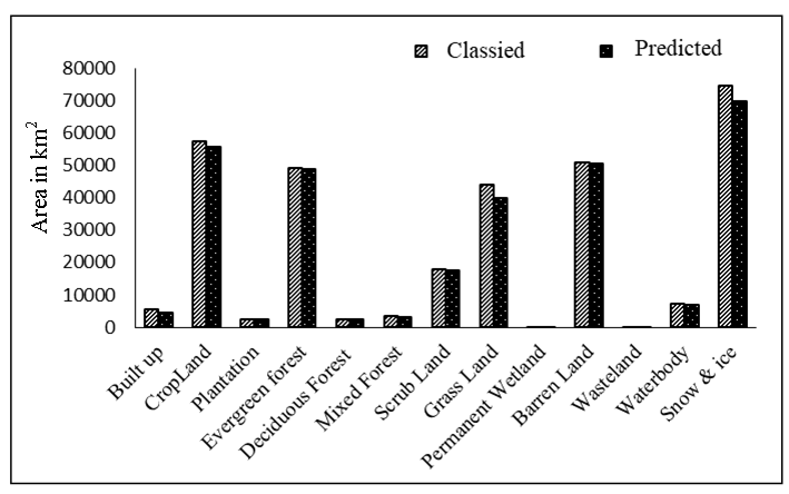
As in the studies conducted by Walsh et al., (2006) and Wu et al., (2006), the parameterization and calibration of the current driver-based statistical model involved a detailed analysis of the historical land use database as developed from Landsat MSS (1985), LISS-I (1995) and LISS-III (2005) and assessing their transition rules in the Markov chain for predicting future land use statistics. The model was also parameterized with a considerable number of driving factors (physical and human induced) that were spatially distributed throughout the study area. Thirteen land use classes were identified from the study area of which the built-up, cropland, vegetation, grassland, barren land and snow and ice classes were significant. Data for four decades (1985, 1995, 2005 and 2015) were available for the Indus watershed, which made the model validation possible. Simulation was implemented for 2005, 2015 and 2025, and validation was accomplished by comparing the performance of the model and the observed changes for 2005 and 2015 (Table 3 and Figure 9).
Figure 9a. Classified and predicted LULC: 2005
Figure 9b. Classified and predicted LULC: 2015
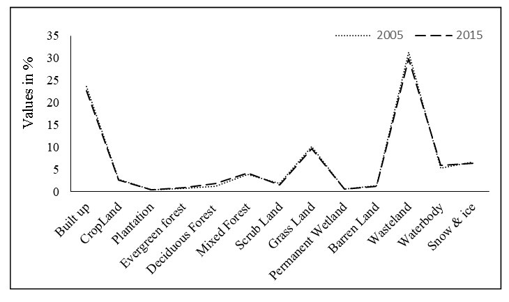
Figure 9c. Prediction error: 2005 and 2015
7 . DISCUSSION
Indus valley, an international river (Indian part includes upstream of the basin) and with a unique physiography has strategic significance for water resources and climate change impacts. Because of its geographical location, the landscape of the Indus river basin is influenced by both physical (slope, climate, soil) and the socio-economic parameters (population growth or socio-economic status). The study evaluates a dynamic land use simulation model (an integration of Markovian transition functions and statistical regressions) developed to predict future land use scenarios of the basin on the basis of its past processes of change. The two main assumptions, followed in the analysis were (1) the best fit relation the drivers have with land use may be projected and (2) that the past trend of change will continue for each class in the future.
Table 3 displays the area statistics of the LULC classes of the classified base year (2005) and the initial years (1985 and 1995) as well as the predicted ones for 2015 and 2025. There was a gradual but significant rise in the built up area, as is evident from the table. There was a major reduction in the acreage of cultivated land with time, which may be due to the urban expansion in agricultural land, or conversion to wasteland and scrubland due to soil fertility depletion (Singh et al., 2010; Bhattacharyya et al., 2015). The area covered by natural vegetation, as an aggregate of evergreen, deciduous and mixed forest, decreased considerably from 2005 due to deforestation. Minor alterations can be seen for plantation and wetlands, where there were slight increases. The area under permanent snow cover also decreased consistently with time, which might be attributed to a considerable rise in temperature due to climate change, and as a consequence the area under waterbodies as well as grassland has increased (Pandey and Venkatraman, 2012).
The similar land use dynamics study by Brown et al., (2000) in the Upper Midwest area of the United States of America, envisaged changes in forest cover with respect to socio-economic changes in the region using a transition matrix and regression models, which indicated that almost 60% of the variations in the transition probability of forest cover can be predicted using human variables such as area under cropland, extent of developed area and rate of development. The Markov modelling technique was also used by Tsarouchi et al., (2014) to successfully generate a future land use scenario in the Upper Ganga basin on the basis of historical records of change from 1984 to 2010.
From the model validation, it was found, for both the years (2015 and 2025), except for built-up land and wastelands, the prediction error was less than 10% (Figure 9). The accuracy of prediction of the model is around 70% for built-up land and wasteland due to the poor scale of data analysis (coarser resolution, 1:250,000). A relatively detailed scale is required to assess the considerable extent of change in these land use classes. At the coarser scale, most of the changes in these classes get masked by the areas under homogenous land use categories, making them barely discernible. Moreover, the wasteland land use class in any region is mostly affected by the present soil condition and the rainfall pattern rather than past patterns in the climate or soil productivity. Although the model is able to predict almost 70% to 90% of the variability in land use classes, the major weakness involves the use of past drivers for predicting future land use. The performance of the model can be improved by considering the dynamic nature of the drivers along with LULC and assessing human land use classes such as built-up land and wasteland at a larger scale and a finer resolution.
Such research outputs i.e. three decades of past land use/ land cover (LULC) maps, their spatial dynamics and simulated future land use maps (of 2015 and 2025) are invaluable inputs to evaluate regional plans for sustainable development. The results of the study provide useful aids for applications in demarcating conservation area, locating regions for ecological restoration, land erosion or degradation, agroforestry or horticulture area zoning and mitigating effects of climate change. The presented approach of LULC change modelling can be used in the similar landscapes of India or elsewhere.
8 . CONCLUSIONS
A LULC change database was generated for the current study at a scale of 1:250,000. It serves the purpose of capturing broad changes in land use, as identified by the past drivers of change, and can be used to recognize areas or identify land use classes where a finer and better-quality database needs to be developed for more detailed investigations and modelling. The approach and the result represented in the present study can be used in the similar landscapes of India or elsewhere. The uniqueness of LULC of Indus river basin is characterized by the natural vegetation in its mountainous landscape, intensive agriculture, expanding settlements in the alluvial plains or valleys and snowy high altitude peaks. The physiography and landforms largely influence the distribution of natural vegetation dominated by forest, grassland or shrub land and human modified landscapes like orchards and degraded forests. Because of the physiographic variability of the Indus basin, both natural and human drivers of change were found to be significant in shaping its landscape. The geographic location of the basin plays an important role in the distribution of land cover and land use classes and their processes of change.
Future distribution of 13 LULC classes over the basin area was modelled using a combination of transition probability and regression equation based on their past pattern of change with an average accuracy of 80 to 85%. Model validation proved that scale is a major dependency of the land use classes for an accurate simulation. Heterogeneous classes like built up or wasteland needs finer scale of assessment to capture their spatial and temporal variability.
Tables
Figures
Conflict of Interest
The authors declare no conflict of interest.
Acknowledgements
The present study has been supported by ISRO Geosphere Biosphere Programme (IGBP) on land- use/land cover dynamics in Indian River basins and impact of human drivers thereof. The authors are thankful to Director, IIRS for all necessary support.
Abbreviations
BL: Barren Land; BU: Built up Area; CL: Cropland; DD: Drainage Density; DF: Deciduous Forest; EF: Evergreen Forest; GL: Grassland; IGBP: International Geosphere and Biosphere Program; IHDP: International Human Dimensions Program; LULC: Land Use Land Cover; MF: Mixed Forest; PL: Plantation; PW: Permanent Wetland; SEI: Socio Economic Index; SEOE: Standard Error of Estimate; SL: Scrub Land; WB: Water-body; WL: Wasteland.
Agarwal, C., Green, G. M., Grove, J. M., Evans, T. P. and Schweik. C. M. 2001. A review and assessment of land-use change models: Dynamics of space, time, and human choice. Bloomington, IN: South-Burlington, Centre for the Study of Institutions Population, and Environmental Change, Indiana University.
IGBP, 1995. Land use and Land cover change. Science/ Research plan (Ed.) Turner B L, Skole D, Sanderson S, Fischer G, Fresco L and Leemans IGBP report 35/ IHDP report 7, Stolkholm and Geneva, IGBP/IHDP
Kumar, M. and Rajan, K.S. 2014. Modelling Land-Use Changes in Godavari River Basin: A Comparison of Two Districts in Andhra Pradesh. 7th Intl. Congress on Environmental Modelling and Software, San Diego, California, USA Daniel P. Ames, Nigel W. T. Quinn, Andrea E. Rizzoli (Eds.).
Parvez, M.R., Madurapperuma, B., and Ripplinger, D. 2015. Modeling Land Use Pattern Change Analysis in the Northern Great Plains: A Novel Approach. In:2015 Agricultural & Applied Economics Association and Western Agricultural Economics Association Annual Meeting, San Francisco, CA, July 26-28.
Pijanowski, B. C., Machemer, T., Gage, S., Long, D., Cooper, W., and Edens, T. 1995. A land transformation model: integration of policy, socioeconomics and ecological succession to examine pollution patterns in watershed. Report to the Environmental Protection Agency, Research Triangle Park, North Carolina. 72.
31.
Pijanowski, B. C., Machemer, T., Gage, S., Long, D., Cooper, W., and Edens, T. 1996. The use of a geographic information system to model land use change in the Saginaw Bay Watershed. Proceedings of the Third International Conference on GIS and Environmental Modeling, Sante Fe, New Mexico, January 21-26, 1996. GIS World Publishers on CD-ROM.
Rashid, A., Sayyed, M. R. G., and Bhat F. A. 2015. The dynamic response of Kolohai Glacier to climate change. Proceedings of the International Academy of Ecology and Environmental Sciences, 5(1), 1-6.
35.
Rawlings, J.O., Pantula, S.G., and Dickey, D.A. 1998. Applied regression analysis: a research tool. (2nd Eds.) Springer-Verlag New York Berlin Heidelberg.


 ,
Parth Sarathi Roy 2
,
Parth Sarathi Roy 2